building a DQN without machine learning libraries

Jan 2026·from scratch·code on GitHub

Modern machine learning frameworks are widespread precisely because they mask the complexity of the algorithms they provide access to. This is almost always a positive factor - it saves time when programming, and avoids errors in original code that could cause a solution to not be properly optimized, or not work at all. With that said, today I would like to take a closer look at what runs behind those abstractions - specifically by building up a neural network from scratch, and looking at one interesting application in deep Q-learning.

I would highly recommend following the repository code as you read through this article. The project is made up of three codebases that stack:

• Neural_network_api - a modular neural-network library built on just NumPy, comprising layers, activations, cost functions, a simple training loop and disk serialisation.
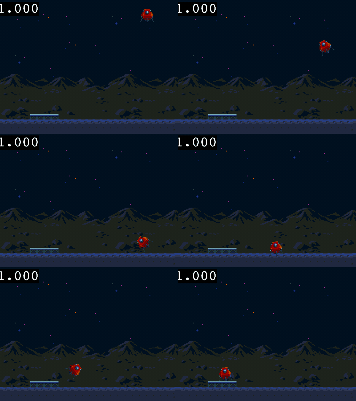
• Environment_maker - a Pygame based 2D rigid-body physics engine, including sprites with mass, inertia, drag and convex-polygon collision detection, as well as an impulse-based collision response. It is an example environment modelled on the OpenAI Gym interface. Put simply - this environment provides a physics-based simulation of a small rocket that can rotate or use thrusters to try and land on a platform which appears in randomized positions at the bottom of the window.
• Lander_environment.py - the Deep Q-Network (DQN) agent, plus the lunar-lander game it learns to play, built from the two libraries above.

Neural networks, briefly

The first part of the theory is understanding neural networks at a very simple level. A feed-forward neural network is a chain of relatively straightforward functions. A fully connected layer (which is what we will be using for the rest of the article) simply multiplies its input row-vector x by a weight matrix W and adds a bias:

$$y = xW + b$$

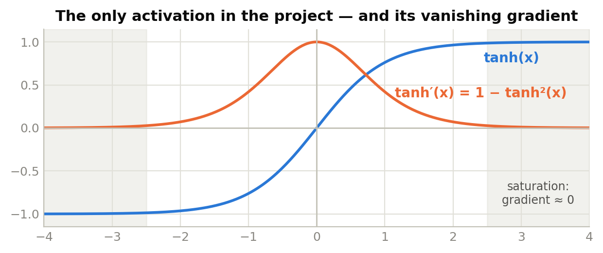
An activation layer is then used to apply an elementwise non-linearity. At first that can read as quite complicated, or perhaps even redundant, but it is just required as without it, stacking linear layers would collapse into a single linear map. This project will use tanh everywhere: it is smooth, symmetric around zero, and its derivative is cheap to compute from the function value itself. The reason why these characteristics are valuable will become clearer after looking at the training loop.

When we talk about training a model, we usually mean changing its parameters so that it is the most accurate model possible. In practice, we apply this as: change the model's parameters so it is the least wrong as possible. To know how 'wrong' the model is on any given answer, we require a cost function. For simplicity, I will implement mean squared error, but it is important to note that the best cost function for a task depends entirely on the task itself. Here, mean squared error (MSE) works well with the penalties that we will implement (which will be expanded on later). In practice, MSE is relatively easy to implement, but if you are interested in the specific formulae, the value and derivative of MSE are:

$$E = \frac{1}{n}\sum_{i=1}^{n}\left(\hat{y}_i - y_i\right)^2, \qquad \frac{\partial E}{\partial \hat{y}_i} = \frac{2}{n}\left(\hat{y}_i - y_i\right)$$

Backpropagation is another important concept. It consists of the chain rule applied layer by layer, backwards. Each layer receives the derivative of the cost with respect to its own output (which you can call δ) and must produce three items: the gradient of its weights, the gradient of its bias, and the derivative with respect to its input, which then becomes δ for the layer below.

Gradient descent (SGD) then nudges every parameter downhill: W ← W − η ∂E/∂W, where η is the learning rate. This is the cornerstone of deep learning. Put simply, it is the equivalent of trying to find a Starbucks - you walk around, and when you see someone holding a Starbucks cup, you walk in the opposite direction that they are walking in. Eventually, by making these small updates, we aim to reach a minimum of loss.

Q-learning, briefly

The second important part of theory is Q-learning. Q-learning, simply put, aims to find the total (future discounted) reward you can expect if you take some action a in state s and act optimally afterwards. Using the Bellman equation, we can turn that into an update rule:

$$Q(s,a) \leftarrow Q(s,a) + \alpha\left[\,r + \gamma \max_{a'} Q(s',a') - Q(s,a)\,\right]$$

This formula may appear complicated at first, but is actually very intuitive: Q(s, a) represents the value that we want to find. We take r, the reward for the current action at the current state - for example, the reward for putting down the right answer on a test is passing the test. We then add the maximum value from all of the actions that we are allowed to take from our current state (multiplied by a temporal discount factor gamma, which makes near term rewards more valuable). This simply means that the value of my current decision in my current position, is the reward it brings + (a discounted) value of the next position, given I play optimally.

This type of reinforcement learning tends to use tables - whereby you have a set number of squares on a grid, and each has a value. The lunar lander environment represents the lander's state as 9 numbers (seven continuous components and two binary foot-contact flags). As such, it is impossible to formulate a table for all of the possible situations.

Instead, we have to use a Deep Q-Network (the fusion of the two theory concepts I have just explained). The DQN replaces the table with a neural network trained to minimize the squared temporal difference error. We can see this in the loss function (which should look vaguely familiar):

$$L(\theta) = \mathbb{E}\left[\left(\,r + \gamma \max_{a'} Q(s', a';\, \theta^{-}) - Q(s, a;\, \theta)\,\right)^{2}\right]$$

However, naively bolting a neural network onto the Bellman update is famously unstable, for two reasons:

1. Correlated data - consecutive frames are nearly identical, so training on them in order violates what is called the i.i.d. assumption (that a set of datapoints are independently and identically distributed). If we recall how weights update, we can see how consecutive losses that point in the same direction can cause issues. The fix is experience replay: store transitions in a buffer and train on random samples, breaking the temporal correlation - the same buffer that becomes a problem for a different reason below.
2. Moving targets - the target for each update, r + γ·max Q(s′, a′), is computed by the same network being trained, so every gradient step moves the thing the network is trying to match. The fix is to compute these targets with a periodically-frozen copy of the network (the θ⁻ in the loss above), so one side of the equation stays still between synchronisations.

Finally, the agent must explore in order to learn effectively. ε-greedy action selection takes a random action with probability ε and the best-known action otherwise, with ε decaying over training from 1.0 towards a small floor.

The engine

The neural network engine is simple and works on Layer and NeuralNetwork. Layer simply allows for forward and backwards propagation (forwards for predictions, backwards for training on its mistakes).

Taking a deeper look at the code reveals several important design choices, such as adding the cost function at network construction time, so that anything can be changed as necessary without having to change the training loop. Additionally, the train function allows for two different batching modes: sequential slices, or random sampling with replacement (which is used by the DQN).

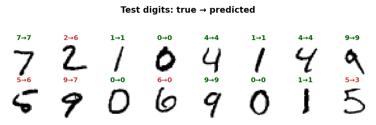
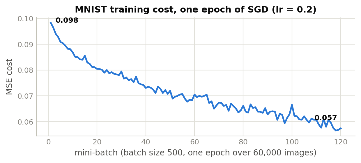
We can test the network on the classic MNIST task (look at an image and decide what digit from 0-9 it is). For reference, a CNN reaches 98%+ here, and even a well-tuned fully-connected network manages around 97% - the gap to my 77% is mostly the MSE loss (cross-entropy is the right choice for classification; recall my note on cost functions) and a deliberately minimal setup. This run is a functionality check, not a benchmark. The results and a few predictions are shown below:

The physics engine is another interesting discussion point, but not within the scope of this post, so I will leave it out for a future post. I would be happy to discuss any questions on the physics (or neural network) engine at my email or contact points that can be found in my about section.

Actually implementing the DQN

What failed

• Sparse rewards - rewarding the agent only for reaching the goal was not a useful strategy, as after thousands of episodes, the agent was still moving around randomly. The takeaway is that an agent can only learn from rewards it can achieve.
• Feeding raw state components - positions in pixels and velocities on completely different scales pushed tanh straight into its saturated region, where gradients vanish. Normalising every component to [-1, 1] fixed it (recall the tanh figure).
• A failure-dominated replay buffer - a buffer was used to hold 'memories' (episodes that would be stored to later be trained on). This buffer (as expected) was swiftly populated with only negative rewards, which made it very hard to train on. This behaviour was so pertinent, that the agent began simply hovering, to avoid the negative rewards.

The fixes

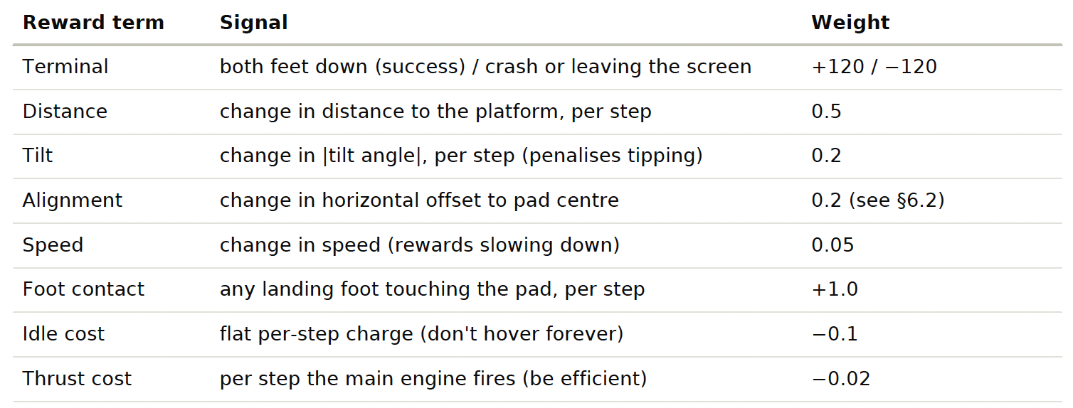
• Reward shaping - pay the agent a small reward for every step it progresses towards the end goal - for example, the agent gained a reward for moving closer to the platform. Each term for these rewards was made up of a change in a state quantity between steps. For example, if the agent slowed down, this decrease in speed would be clamped (so that no large increase or decrease in speed could dominate the term) and then multiplied by some reward term. It is important to note that the end reward should always be the largest reward, as it is the end goal which the agent is actually made to pursue in practice.

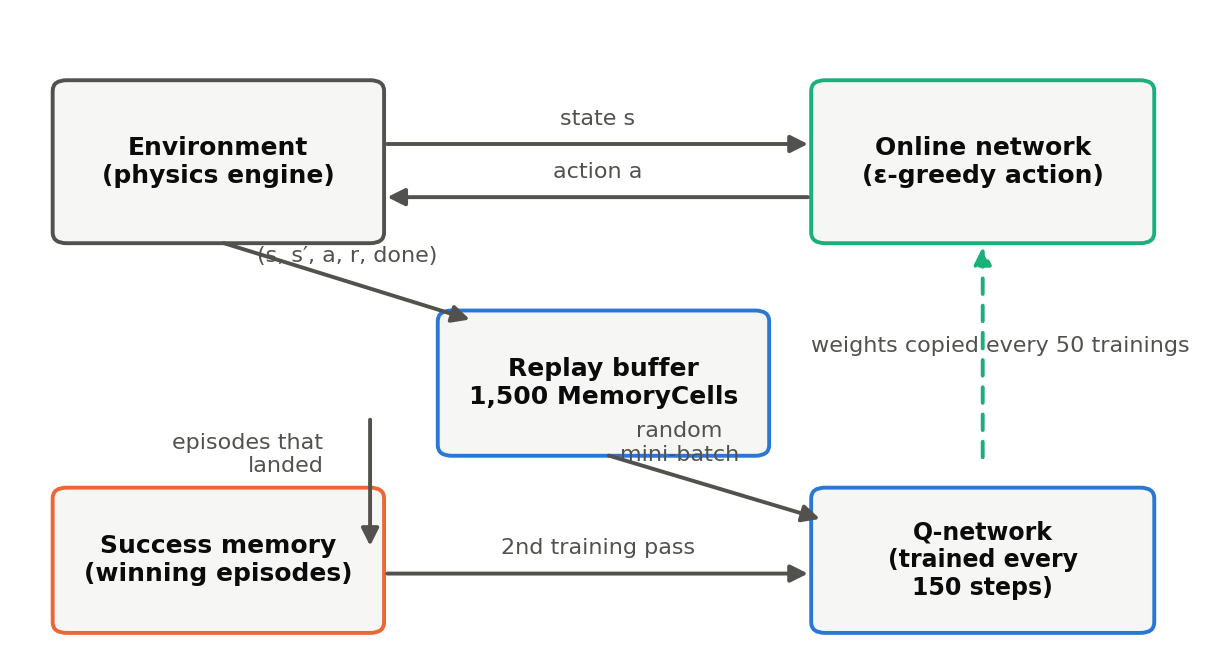
• A separate buffer for success - to beat the failure-dominated buffer, the agent maintains a second list made up of episodes which ended with positive terminal rewards. Each training round makes two passes: a random mini-batch over the ordinary buffer, followed by a second, smaller-batch pass over the accumulated successes.

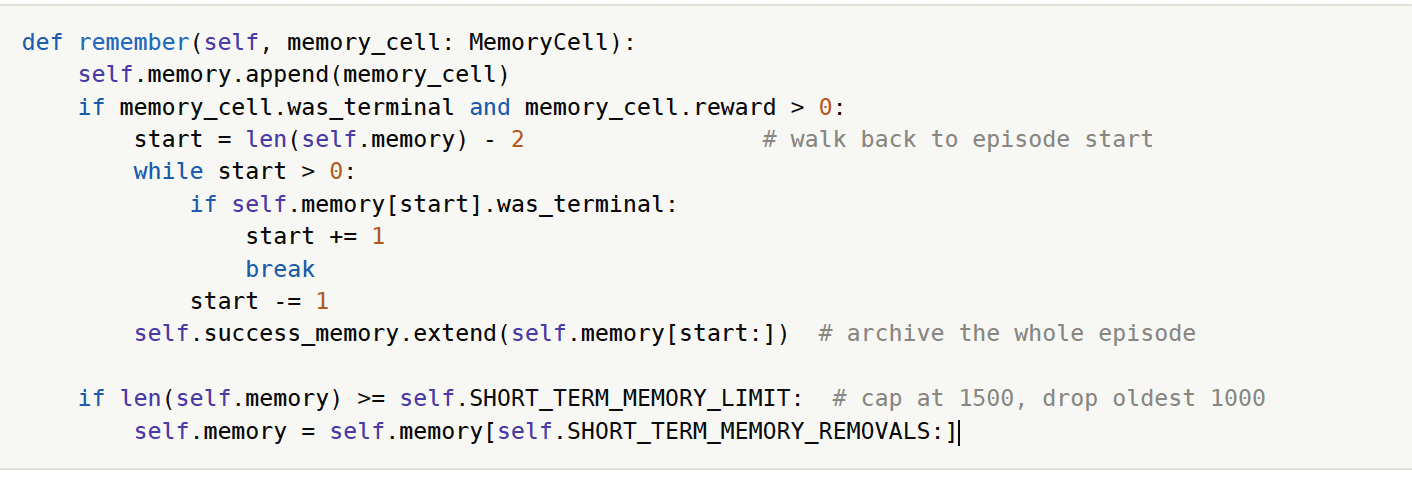
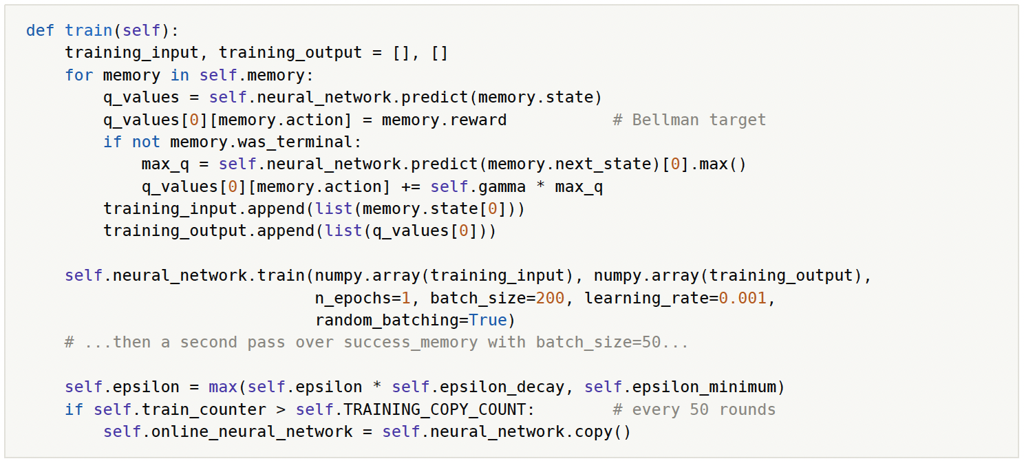
Training builds a supervised dataset from memory: for each remembered transition, predict the current Q-values, overwrite the entry for the action actually taken, and fit the network to the result with the same MSE and backpropagation used for MNIST. Two network copies are used: a frozen copy drives ε-greedy action selection, refreshed only every 50 training rounds, so that the behaviour policy stays stable while the trained network changes. Note that this inverts the usual DQN recipe, where the frozen copy computes the update targets while the acting network learns; here the update targets come from the live network. The consequences of that inversion turn out to matter, and the results below return to it.

Debugging a Deep Q-Network

Debugging a DQN is a relatively challenging task - errors tend to not be NaNs, or exceptions, but instead just an agent that fails to learn effectively. When this is combined with the naturally long training times, debugging effectively can become a real challenge.

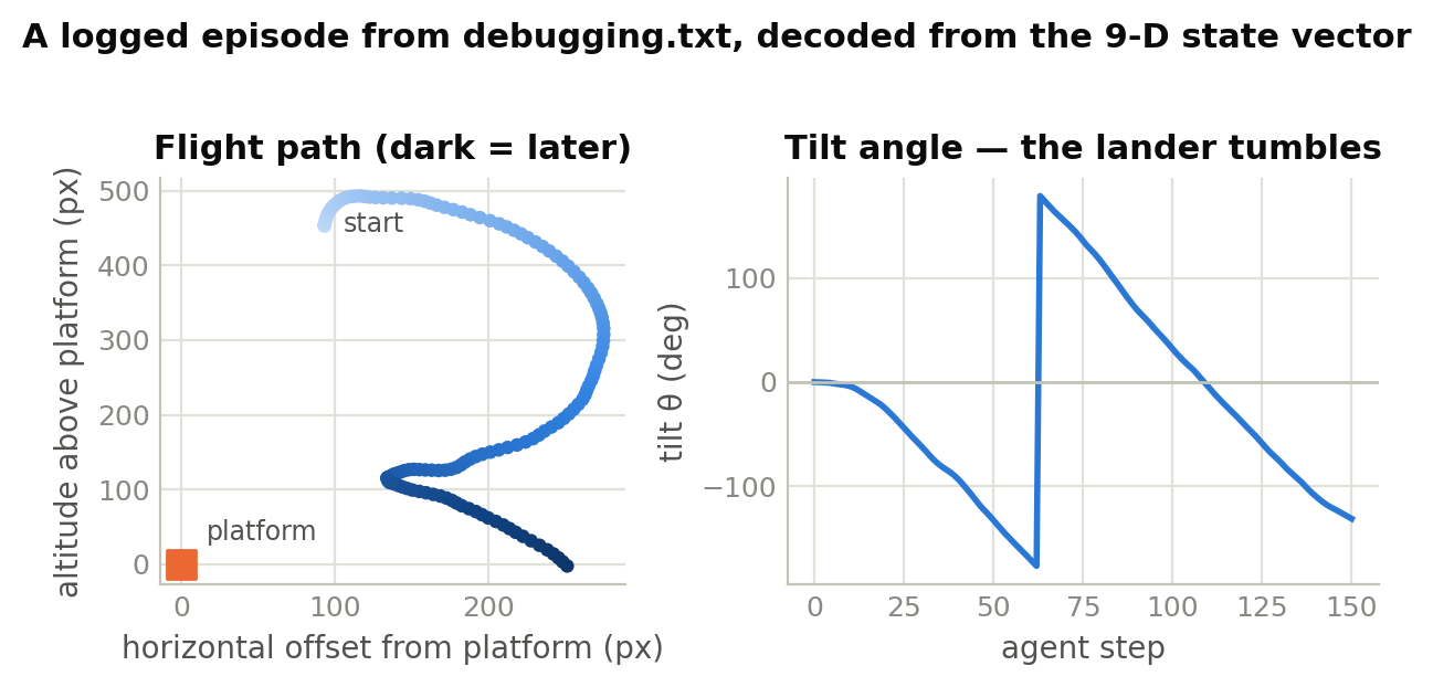
Even with good reward shaping, the full task (which incorporates the lander spawning anywhere and the random platform spawning) was too challenging to learn from scratch. A solution that worked was curriculum learning, whereby the task starts easy and is gradually made more difficult every time the agent reached a specific number of successes.

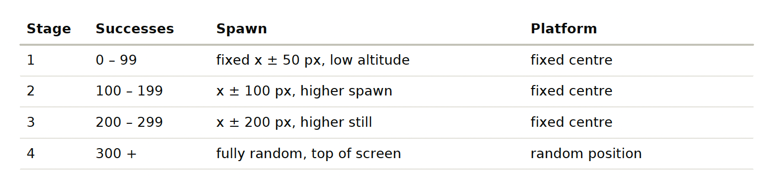
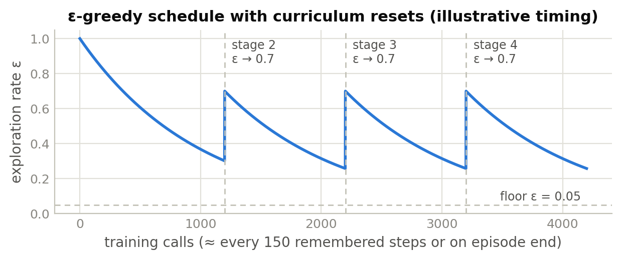
After each new stage in the curriculum, the value for ε (the 'randomness' factor) is reset to 0.7, so that the agent continues to explore in its new environment. The curriculum keeps successes frequent enough to fill the success memory buffer, and the ε value resets keep the buffer supplied with fresh experience of each new difficulty tier.

Takeaways

• Backpropagation is not that complicated - often everything is hidden behind a .backward() call, which can feel quite opaque. Understanding the value of gradients through backpropagation enables being more comfortable using them in other contexts, such as the application of a Fisher information matrix for Elastic Weight Consolidation (which is an important construct when training the same model on a second task, when you do not want it to forget the first).
• Reinforcement learning's primary error case is a failure to learn - there are many solutions to this, a handful of which are covered in this article. The important takeaway is that if a reward is too difficult to achieve, or the model sees every scenario as negative, it will end up just avoiding the larger negative, which often produces behaviours that are unwanted.

The system is naturally a relatively basic baseline, with some interesting examples of techniques to improve the network. You can easily explore further by changing the environment or tweaking the network.

Referenced papers for further reading

Rumelhart, D. E., Hinton, G. E. & Williams, R. J. (1986). Learning representations by back-propagating errors. Nature 323.

Lin, L.-J. (1992). Self-Improving Reactive Agents Based on Reinforcement Learning, Planning and Teaching. Machine Learning 8.

Watkins, C. J. C. H. & Dayan, P. (1992). Q-learning. Machine Learning 8.

Ng, A. Y., Harada, D. & Russell, S. (1999). Policy Invariance Under Reward Transformations: Theory and Application to Reward Shaping. ICML 1999.

Bengio, Y., Louradour, J., Collobert, R. & Weston, J. (2009). Curriculum Learning. ICML 2009.

Mnih, V. et al. (2015). Human-level control through deep reinforcement learning. Nature 518. arXiv:1312.5602.

Kirkpatrick, J. et al. (2017). Overcoming catastrophic forgetting in neural networks. PNAS 114(13). arXiv:1612.00796.